Universal Decomposition of Perturbation Effects

In this tutorial, we will systematically analyze a perturb-seq dataset by decomposing the perturbation effects on to the globally defined principal axes of cell state transitions.

import numpy as np
import pandas as pd
import scipy
import matplotlib.pyplot as plt

import scanpy as sc

Load and preprocess the perturb-seq dataset

Load the example perturb-seq dataset. This is a CRISPRi dataset.

adata = sc.read_h5ad('data/tutorial_data/AdamsonWeissman2016_GSM2406681_10X010.h5ad')
adata

AnnData object with n_obs × n_vars = 65337 × 32738
    obs: 'perturbation', 'read count', 'UMI count', 'tissue_type', 'cell_line', 'cancer', 'disease', 'perturbation_type', 'celltype', 'organism', 'ncounts', 'ngenes', 'percent_mito', 'percent_ribo', 'nperts'
    var: 'ensembl_id', 'ncounts', 'ncells'

Normalize the total count of each cell

sc.pp.normalize_total(adata, target_sum=1e4)

Let’s have a look at what genes are perturbed in this dataset and the number of cells for each perturbation.

condition_col = 'perturbation'
condition_cell_counts = adata.obs[condition_col].value_counts()
for c in condition_cell_counts.index:
    print(f'{c}\t{condition_cell_counts.loc[c]}')

63(mod)_pBA580  6010
Gal4-4(mod)_pBA582      1283
IER3IP1_pDS002  1222
SEC61B_pDS033   1185
ASCC3_pDS052    1142
DNAJC19_pDS026  1000
HSPA9_pDS088    894
HSPA5_pDS017    881
YIPF5_pDS186    817
SAMM50_pDS156   817
TARS_pDS405     803
XRN1_pDS411     788
GBF1_pDS043     760
TIMM23_pDS284   757
DAD1_pDS499     752
SEC61A1_pDS032  740
AMIGO3_pDS434   715
SRPRB_pDS404    703
SRP68_pDS403    699
UFM1_pDS040     692
TELO2_pDS496    691
FECH_pDS494     683
MRPL39_pDS498   683
IARS2_pDS091    673
SCYL1_pDS160    669
DARS_pDS495     664
IDH3A_pDS393    663
DERL2_pDS042    656
SEC63_pDS218    654
TTI2_pDS408     653
SYVN1_pDS442    650
SEC61G_pDS440   650
SPCS3_pDS402    647
OST4_pDS353     646
ATP5B_pDS055    644
SLMO2_pDS433    637
FARSB_pDS390    632
TMED10_pDS036   626
PSMD4_pDS488    625
EIF2B4_pDS491   625
SLC35B1_pDS046  621
EIF2B2_pDS463   615
ASCC3_pDS051    614
DDRGK1_pDS041   607
GMPPB_pDS391    606
SLC39A7_pDS219  601
SRPR_pDS482     591
TIMM44_pDS430   590
SPCS2_pDS401    587
UFL1_pDS410     585
PDIA6_pDS029    583
IER3IP1_pDS110  582
YIPF5_pDS226    574
MRGBP_pDS124    570
SCYL1_pDS159    561
P4HB_pDS397     560
MANF_pDS027     554
PTDSS1_pDS478   534
TTI1_pDS407     526
DNAJC19_pDS074  525
MARS_pDS394     523
SRP72_pDS505    520
MTHFD1_pDS395   520
EIF2S1_pDS386   511
DHDDS_pDS383    507
NEDD8_pDS396    506
TMED2_pDS175    505
GNPNAT1_pDS506  503
CARS_pDS460     501
STT3A_pDS011    499
HYOU1_pDS089    494
ARHGAP22_pDS458 490
SEC61B_pDS162   483
CHERP_pDS024    479
SARS_pDS467     473
TMEM167A_pDS038 468
KCTD16_pDS096   464
SEC61A1_pDS031  451
SOCS1_pDS479    450
AARS_pDS381     447
SEL1L_pDS373    443
IARS2_pDS090    438
EIF2B3_pDS508   415
HSD17B12_pDS087 404
DDOST_pDS382    382
CCND3_pDS006    379
QARS_pDS510     379
HARS_pDS466     325
ATF4_pBA608     325
HSPA5_pDS371    301
COPZ1_pDS462    282
CAD_pDS468      281
PPWD1_pDS398    234
COPB1_pDS065    225
GBF1_pDS044     198
EIF2AK3_pBA572  141
*       101
PSMD12_pDS008   49
ERN1_pBA575     43
ERN1_pBA574     40
XBP1_pBA579     34
PSMA1_pDS007    29
XBP1_pBA578     28
IER3IP1_pDS003  26
ATF4_pBA577     23
EIF2AK3_pBA573  20
CCND3_pDS005    18
C7orf26_pDS004  12
PSMD12_pDS009   11
ATF6_pBA586     10
YIPF5_pDS001    9
ATF4_pBA576     5
62(mod)_pBA581  2
STT3A_pDS010    1

Let’s perform a quality control. Let’s filter out perturbation with too few cells and perturbations that don’t effectively knock down the target genes.

control_condition = '63(mod)_pBA580' # The control condition
n_cell_threshold = 100 # The minimum number of cells required for a condition to be considered
perturbation_dict = {
    'condition' : [],
    'perturbed_gene' : [],
    'control_condition': [],
    'fc': [],
    'pval': [],
}

for c in condition_cell_counts.index:

    # Ignore conditions with too few cells
    if condition_cell_counts.loc[c] < n_cell_threshold:
        continue

    # Extract the perturbed genes from the condition name
    perturbed_genes = c.split('_')
    perturbed_genes = np.intersect1d(perturbed_genes, adata.var.index)

    # Only consider single gene perturbations
    if len(perturbed_genes) != 1:
        continue
    pg = perturbed_genes[0]

    # Get the expression of the perturbed gene in the control and perturbed conditions
    control_exps = adata[adata.obs[condition_col] == control_condition, pg
                         ].X.toarray().reshape(-1)
    perturbed_exps = adata[adata.obs[condition_col] == c, pg
                           ].X.toarray().reshape(-1)

    # Calculate the fold-change and p-val for the perturbed gene
    fc = np.mean(perturbed_exps) / np.mean(control_exps)
    pval = scipy.stats.mannwhitneyu(control_exps, perturbed_exps, alternative='two-sided')[1]

    # Only keep the perturbations that are effective
    if (fc < 0.8) and (pval < 1e-2):
        perturbation_dict['condition'].append(c)
        perturbation_dict['perturbed_gene'].append(pg)
        perturbation_dict['control_condition'].append(control_condition)
        perturbation_dict['fc'].append(fc)
        perturbation_dict['pval'].append(pval)


perturbation_df = pd.DataFrame(perturbation_dict).set_index('condition')
perturbation_df

/tmp/ipykernel_752705/3671995774.py:33: RuntimeWarning: invalid value encountered in scalar divide
  fc = np.mean(perturbed_exps) / np.mean(control_exps)

	perturbed_gene	control_condition	fc	pval
condition
SEC61B_pDS033	SEC61B	63(mod)_pBA580	0.173211	0.000000e+00
ASCC3_pDS052	ASCC3	63(mod)_pBA580	0.117991	1.549447e-94
DNAJC19_pDS026	DNAJC19	63(mod)_pBA580	0.162940	0.000000e+00
HSPA9_pDS088	HSPA9	63(mod)_pBA580	0.287186	1.990341e-254
HSPA5_pDS017	HSPA5	63(mod)_pBA580	0.462840	4.543529e-96
...	...	...	...	...
COPZ1_pDS462	COPZ1	63(mod)_pBA580	0.306617	2.228928e-69
CAD_pDS468	CAD	63(mod)_pBA580	0.211891	2.448909e-17
PPWD1_pDS398	PPWD1	63(mod)_pBA580	0.305571	1.135729e-08
COPB1_pDS065	COPB1	63(mod)_pBA580	0.503718	1.162430e-07
GBF1_pDS044	GBF1	63(mod)_pBA580	0.331636	2.903447e-04

87 rows × 4 columns

Next, we compute the pseudo-bulk expression profile of each condition.

from tqdm import tqdm

def get_cluster_mean_expression_matrix(adata, cluster_column):
    '''Get a dataframe of mean gene expression of each cluster.'''
    cluster_names = np.unique(adata.obs[cluster_column].values)
    cluster_mean_df = pd.DataFrame(np.zeros((len(cluster_names), adata.shape[1]), dtype=np.float32),
                                   index=cluster_names, columns=adata.var.index)

    for c in tqdm(cluster_names):
        X_c = adata[adata.obs[cluster_column] == c].X
        cluster_mean_df.loc[c] = X_c.mean(axis=0)

    return cluster_mean_df

# Get mean expressions of each condition
selected_conditions = np.unique(list(perturbation_df.index)
                                + list(perturbation_df['control_condition']))
adata_selected = adata[adata.obs[condition_col].isin(selected_conditions)]

condition_mean_exp_df = get_cluster_mean_expression_matrix(adata_selected,
                                                           condition_col)
condition_mean_exp_df

100%|██████████| 88/88 [00:43<00:00,  2.04it/s]

gene_symbol	MIR1302-10	FAM138A	OR4F5	RP11-34P13.7	RP11-34P13.8	AL627309.1	RP11-34P13.14	RP11-34P13.9	AP006222.2	RP4-669L17.10	...	KIR3DL2-1	AL590523.1	CT476828.1	PNRC2-1	SRSF10-1	AC145205.1	BAGE5	CU459201.1	AC002321.2	AC002321.1
63(mod)_pBA580	0.000000	0.0	0.0	0.0	0.000095	0.003224	0.0	0.0	0.000555	0.0	...	0.0	0.0	0.0	0.000388	0.009653	0.0	0.0	0.0	0.0	0.0
AARS_pDS381	0.000000	0.0	0.0	0.0	0.000000	0.006999	0.0	0.0	0.000964	0.0	...	0.0	0.0	0.0	0.000000	0.011662	0.0	0.0	0.0	0.0	0.0
ARHGAP22_pDS458	0.000000	0.0	0.0	0.0	0.003068	0.002012	0.0	0.0	0.000000	0.0	...	0.0	0.0	0.0	0.000000	0.011770	0.0	0.0	0.0	0.0	0.0
ASCC3_pDS051	0.000000	0.0	0.0	0.0	0.000000	0.003492	0.0	0.0	0.000000	0.0	...	0.0	0.0	0.0	0.000000	0.008839	0.0	0.0	0.0	0.0	0.0
ASCC3_pDS052	0.000000	0.0	0.0	0.0	0.001639	0.002893	0.0	0.0	0.001667	0.0	...	0.0	0.0	0.0	0.000000	0.012430	0.0	0.0	0.0	0.0	0.0
...	...	...	...	...	...	...	...	...	...	...	...	...	...	...	...	...	...	...	...	...	...
UFL1_pDS410	0.000000	0.0	0.0	0.0	0.000000	0.001283	0.0	0.0	0.000000	0.0	...	0.0	0.0	0.0	0.000954	0.009231	0.0	0.0	0.0	0.0	0.0
UFM1_pDS040	0.000432	0.0	0.0	0.0	0.000763	0.000000	0.0	0.0	0.000000	0.0	...	0.0	0.0	0.0	0.000000	0.009446	0.0	0.0	0.0	0.0	0.0
XRN1_pDS411	0.000000	0.0	0.0	0.0	0.002461	0.005934	0.0	0.0	0.000889	0.0	...	0.0	0.0	0.0	0.000000	0.011627	0.0	0.0	0.0	0.0	0.0
YIPF5_pDS186	0.000000	0.0	0.0	0.0	0.000000	0.006665	0.0	0.0	0.000000	0.0	...	0.0	0.0	0.0	0.000531	0.011071	0.0	0.0	0.0	0.0	0.0
YIPF5_pDS226	0.000000	0.0	0.0	0.0	0.000000	0.004654	0.0	0.0	0.001430	0.0	...	0.0	0.0	0.0	0.001212	0.015296	0.0	0.0	0.0	0.0	0.0

88 rows × 32738 columns

Now we can compute the pseudo-bulk perturbation-induced gene expression shift vector for each perturbation.

import anndata

X_perturb = []

# Iterate through the perturbations
for c in tqdm(perturbation_df.index):

    # Compute the log1p normalized mean expression of the perturbed and control conditions
    control_c = perturbation_df.loc[c, 'control_condition']
    x_pert = condition_mean_exp_df.loc[c].values.astype(np.float32)
    x_ctl = condition_mean_exp_df.loc[control_c].values.astype(np.float32)
    x_pert = np.log1p(x_pert / x_pert.sum() * 1e4)
    x_ctl = np.log1p(x_ctl / x_ctl.sum() * 1e4)

    # Compute the difference in mean expression between the perturbed and control conditions
    X_perturb.append(x_pert - x_ctl)

X_perturb = np.array(X_perturb)

# Create the perturbation anndata
adata_perturb = anndata.AnnData(
    X=X_perturb,
    obs=perturbation_df.copy(),
    var=adata.var.copy(),
)

adata_perturb

100%|██████████| 87/87 [00:00<00:00, 1193.11it/s]

AnnData object with n_obs × n_vars = 87 × 32738
    obs: 'perturbed_gene', 'control_condition', 'fc', 'pval'
    var: 'ensembl_id', 'ncounts', 'ncells'

Project perturbation effects onto the principal axes of cell state transitions

Let’s mask out the direct target genes of each perturbation to focus on the downstream effect of the perturbed genes.

# Mask out the direct target genes
for i in range(adata_perturb.shape[0]):
    pg = adata_perturb.obs['perturbed_gene'].iloc[i]

    if pg in adata_perturb.var_names:
        adata_perturb.X[i, adata_perturb.var_names.get_loc(pg)] = 0

Now we can compute the gene expression program shift scores for the globally defined gene expression programs, which represent the principal axes of cell state transitions.

# Load the pre-defined global gene expression programs
gene_exp_cluster_df = pd.read_csv('data/tutorial_data/gene_exp_program_annotation.csv', index_col=0).set_index('gene_name')
adata_perturb.var['gene_exp_cluster'] = gene_exp_cluster_df['cluster_name']

# Initialize the gene program matrix
adata_perturb.uns['gene_program_names'] = list(gene_exp_cluster_df['cluster_name'].unique())
adata_perturb.obsm['gene_program'] = np.zeros((adata_perturb.shape[0], len(adata_perturb.uns['gene_program_names'])))

# Compute the gene program matrix
for i in range(len(adata_perturb.uns['gene_program_names'])):
    genes = list(gene_exp_cluster_df[gene_exp_cluster_df['cluster_name'] == adata_perturb.uns['gene_program_names'][i]].index)
    genes = np.intersect1d(genes, adata_perturb.var_names)
    if len(genes) == 0:
        continue
    scale_factor = np.sqrt(len(genes))
    adata_perturb.obsm['gene_program'][:, i] = scale_factor * np.mean(adata_perturb[:, genes].X, axis=1)

Let’s define the order of the gene expression programs to plot.

gene_program_order = [
    'chromatin structure', 'DNA replication/repair', 'cell cycle (G1/S)', 'cell cycle (prometaphase)', 'cell cycle (M phase)',
    'spliceosome', 'proliferation',
    'ribosome biogenesis', 'ribosomal protein genes', 'mitochondrial encoded', 'cholesterol biosynthesis', 'mitochondrial ribosome',
    'Golgi vesicle transport', 'unfolded protein response',
    'integrated stress response', 'p53 signaling', 'lysosome/autophagy',
    'pluripotency', 'Hox genes', 'glia', 'neural development', 'neuronal', 'peripheral neurons',
    'visual perception', 'retinal epithelium', 'melanin biosynthesis',
    'epithelial', 'respiratory epithelium', 'kidney', 'intestine', 'pancreatic', 'pancreatic islet', 'liver', 'epidermal',
    'mesothelial', 'adipocyte',  'mesenchymal', 'smooth muscle', 'endothelial', 'bone',
    'interferon signaling', 'TNF signaling', 'immune system', 'myeloid', 'macrophage', 'B cell', 'T cell', 'natural killer',
    'mast cell', 'erythroid', 'megakaryocyte',
    'muscle', 'heart', 'cilia',
    ]

Now we can comprehensively plot how each perturbation from this dataset push the cell state to change along each principal axis.

fig, ax = plt.subplots(figsize=(25, 4))

# Plot a column for each expression program
for i in range(len(gene_program_order)):
    x = i - 0.25 + (np.arange(adata_perturb.shape[0]) / adata_perturb.shape[0] / 2)

    idx = adata_perturb.uns['gene_program_names'].index(gene_program_order[i])
    y = adata_perturb.obsm['gene_program'][:, idx]

    ax.axvline(i, color='lightgray', lw=0.5, zorder=-1)
    ax.scatter(x, y, s=1, edgecolor='none', c='gray', rasterized=True)

    # Highlight the top and bottom 3 perturbations
    top_shift_indices = list(np.argsort(y)[:3]) + list(np.argsort(y)[-3:])
    for j in top_shift_indices:
        if np.abs(y[j]) > 0.5:
            ax.text(x[j], y[j], adata_perturb.obs['perturbed_gene'].iloc[j], fontsize=10)
            ax.scatter(x[j], y[j], s=6, edgecolor='red', c='none', linewidth=0.8)
            #print(gene_program_order[i], adata_perturb.obs['perturbed_gene_name'].iloc[j], f'{y[j]:.2f}')


ax.axhline(0, color='lightgray', lw=0.5, zorder=-1)
ax.set_xticks(np.arange(len(gene_program_order)), gene_program_order, rotation=45, ha='right')
ax.set_xlim(-1, len(gene_program_order))
ax.set_xlabel('Gene Expression Programs')
ax.set_ylabel('Program Activity')

plt.show()

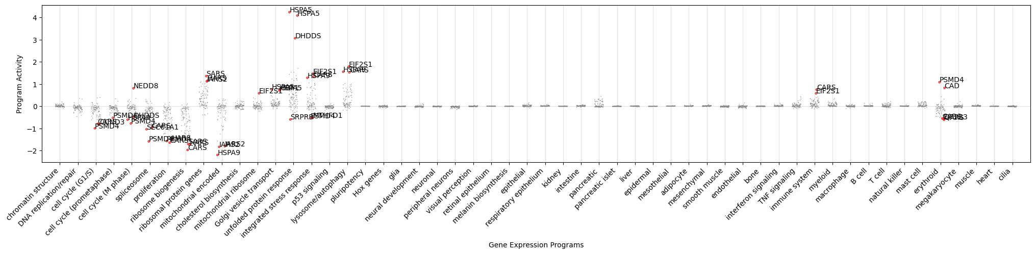
Here we can see that the major effect of perturbations are turning on stress response pathways and turning down essential programs such as spliceosome and ribosome biogenesis. But we can also find a few examples, such as PSMD4, that affect the differentiation state of the cell along the erythroid axis.

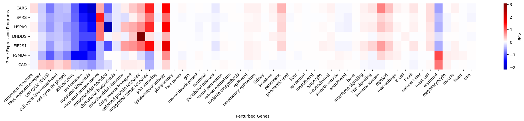
We can zoom-into the interesting genes to comprehensively visualize their perturbation effects along major axes of cell state transition.

genes_to_show = [
   'CARS', 'SARS', 'HSPA9', 'DHDDS', 'EIF2S1', 'PSMD4', 'CAD',
     ]

adata_to_show = adata_perturb[adata_perturb.obs['perturbed_gene'].isin(genes_to_show)].copy()
genes_to_show = [g for g in genes_to_show if g in adata_to_show.obs['perturbed_gene'].values]

gene_program_show_df = pd.DataFrame(
    index=adata_to_show.obs['perturbed_gene'],
    columns=adata_to_show.uns['gene_program_names'],
    data=adata_to_show.obsm['gene_program']
)


fig, ax = plt.subplots(figsize=(25, 3))

import seaborn as sns
sns.heatmap(gene_program_show_df.loc[genes_to_show, gene_program_order], cmap='seismic', ax=ax, center=0,
            cbar_kws={'label': 'RMS'})
ax.set_xticklabels(ax.get_xticklabels(), rotation=45, ha='right')

ax.set_xlabel('Perturbed Genes')
ax.set_ylabel('Gene Expression Programs')

Text(283.22222222222223, 0.5, 'Gene Expression Programs')

We can check the perturbation-induced expression of individual genes to validate the collective phenotypes such as the erythroid differentiation caused by PSMD4 and CAD perturbation.

Let’s plot all the genes belonging to the erythroid program.

perturbed_genes_to_show = [
    'PSMD4', 'CAD',

]
perturbed_genes_to_show = [g for g in perturbed_genes_to_show if g in adata_perturb.obs['perturbed_gene'].values]
perturbed_gene_ids = [list(adata_perturb.obs['perturbed_gene']).index(g) for g in perturbed_genes_to_show]

target_genes_to_show = sorted(adata_perturb.var[adata_perturb.var['gene_exp_cluster'] == 'erythroid'
                                                ].index.values)

target_gene_ids = [list(adata_perturb.var.index).index(g) for g in target_genes_to_show]

mtx = adata_perturb.X[perturbed_gene_ids, :][:, target_gene_ids]

fig, ax = plt.subplots(figsize=(15, 2))
sns.heatmap(mtx, cmap='coolwarm', center=0, vmin=-0.5, vmax=0.5,
              xticklabels=target_genes_to_show, yticklabels=perturbed_genes_to_show,
              cbar_kws={'label': 'gene expression shift'},)
plt.xlabel('Readout genes')
plt.ylabel('Perturbed genes')

Text(158.22222222222223, 0.5, 'Perturbed genes')

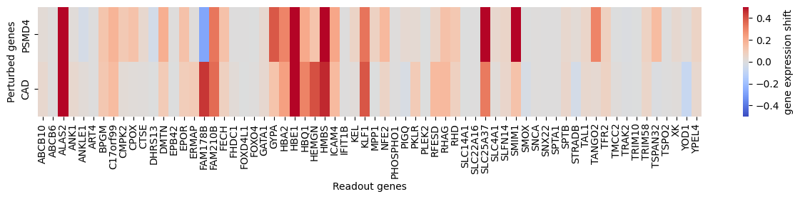
Indeed, we can see specific marker genes of erythrocytes, such as the hemoglobins (HBA2, HBE1 and HBQ1) and the transcription factor KLF1, being upregulated by knocking down PSMD4 and CAD.

Grouping of perturbations into universal clusters

So far we have analyzed the principal phenotypes of individual perturbations. We can further gain a comprehensive picture of the coupling between different cellular processes and phenotypes by grouping perturbations into the pre-defined universal clusters.

Let’s load the pre-defined clusters and compute the mean perturbation effects of each cluster.

pert_cluster_df = pd.read_csv('data/tutorial_data/perturbation_cluster_annotation.csv', index_col=0)
pg_to_cluster_map = dict(zip(pert_cluster_df['perturbed_gene_name'], pert_cluster_df['cluster_name']))

adata_perturb.obs['cluster_name'] = adata_perturb.obs['perturbed_gene'].map(pg_to_cluster_map)
perturb_group_df = pd.DataFrame(
    index=list(adata_perturb.obs[~adata_perturb.obs['cluster_name'].isna()]['cluster_name'].unique()),
    columns=adata_perturb.uns['gene_program_names'],
    dtype=float,
)

for pg_cluster in perturb_group_df.index:
    pg_genes = list(adata_perturb.obs[adata_perturb.obs['cluster_name'] == pg_cluster].index)
    perturb_group_df.loc[pg_cluster] = adata_perturb[pg_genes].obsm['gene_program'].mean(axis=0)

Let’s plot how each perturbation cluster affect the expression of the essential gene expression programs.

pg_cluster_order = [
    'chromatin organization', 'DNA replication', 'histone acetylation', 'CCT complex',
    'mediator complex', 'transcription initiation', 'integrator complex', 'pol II transcription', 'pol II enlongation',
    'spliceosome', 'RNA metabolism', 'RNA degradation', 'RNA methylation', 'mRNA Polyadenylation', 'mRNA surveillance',
    'ribosome small unit biogenesis',
    'ribosome small unit protein', 'rRNA processing 1', 'rRNA processing 2',
    'ribosome large unit biogenesis', 'ribosome large unit protein',
    'translation initiation', 'Recycling Of eIF2:GDP',
    'protein neddylation', 'proteasome',
    'protein processing in ER', 'membrane fission',
    'mitochondrion organization', 'mitochondrial translation', 'mitochondrial transcription',
]
pg_cluster_order = [c for c in pg_cluster_order if c in perturb_group_df.index]

gene_program_order = [
    'chromatin structure', 'DNA replication/repair', 'cell cycle (G1/S)', 'cell cycle (prometaphase)', 'cell cycle (M phase)',
    'spliceosome', 'proliferation',
    'ribosome biogenesis', 'ribosomal protein genes', 'mitochondrial encoded', 'cholesterol biosynthesis', 'mitochondrial ribosome',
    'Golgi vesicle transport', 'unfolded protein response',
    'integrated stress response', 'p53 signaling', 'lysosome/autophagy',

    ]


fig, ax = plt.subplots(figsize=(8, 8))
sns.heatmap(perturb_group_df.loc[pg_cluster_order, gene_program_order],
            cmap='seismic', center=0, cbar_kws={'label': 'mean gene program shift'},
            #xticklabels=False, yticklabels=False,
            vmax=2, vmin=-2,
            ax=ax
            )

ax.set_xticklabels(ax.get_xticklabels(), rotation=45, ha='right')
ax.set_xlabel('Gene expression programs')
ax.set_ylabel('Functional clusters')

Text(70.7222222222222, 0.5, 'Functional clusters')

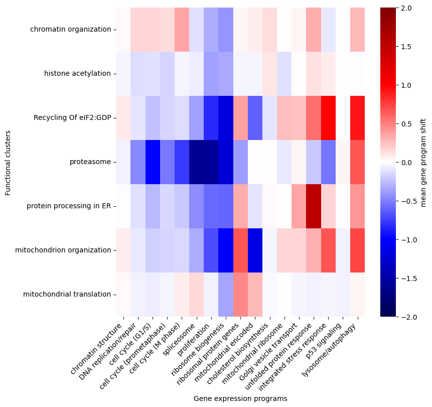
Several interesting patterns emerge:

1. Proliferation related processes including DNA replication/repair, cell cycle (G1/S), cell cycle (prometaphase), cell cycle (M phase), spliceosome, proliferation and ribosome biogenesis are broadly turned down by diverse perturbations, suggesting perturbation-induced cell cycle arrest.

2. Unlike ribosome biogenesis, which is co-regulated with genes for proliferation, the ribosomal protein genes are regulated with a different pattern, suggesting its responsibility for maintaining other aspects of cellular homeostasis.

3. Stress response pathways are activated by distinct spectra of perturbations. As expected, K562 cells have no p53 signaling. Several perturbation clusters, including recycling of eIF2:GDP, protein processing in ER and mitochondrion organization can activate multiple pathways, including unfolded protein response, integrated stress response and lysosome/autophagy pathways. But perturbation of proteasome selectively activate lysosome/autophagy.